确定性规划
确定性规划是指在状态转移完全确定的环境中进行规划。本章将介绍确定性规划的核心概念和算法。
学习目标
完成本章后,你将能够:
- 理解状态空间搜索的基本概念
- 掌握前向搜索和后向搜索方法
- 理解启发式搜索的原理
- 掌握规划空间搜索方法
1. 状态空间搜索
1.1 前向搜索(前进搜索)
前向搜索从初始状态开始,逐步应用动作,直到达到目标状态。
import heapq

def forward_search(problem, heuristic=None):
    """
    前向搜索

    参数:
    problem: 规划问题
    heuristic: 启发函数

    返回:
    plan: 动作序列
    """
    # 初始化
    frontier = [(0, problem.initial_state)]
    explored = set()
    parent = {problem.initial_state: None}
    action_taken = {problem.initial_state: None}
    g_score = {problem.initial_state: 0}

    while frontier:
        f, state = heapq.heappop(frontier)

        if problem.is_goal(state):
            # 重建路径
            plan = []
            while state is not None:
                if action_taken[state] is not None:
                    plan.append(action_taken[state])
                state = parent[state]
            return plan[::-1]

        if state in explored:
            continue

        explored.add(state)

        # 扩展状态
        for action in problem.get_applicable_actions(state):
            new_state = action.apply(state)
            new_g = g_score[state] + 1  # 假设每步代价为1

            if new_state not in g_score or new_g < g_score[new_state]:
                g_score[new_state] = new_g

                # 计算 f 值
                if heuristic:
                    h = heuristic(new_state, problem.goal_state)
                else:
                    h = 0
                f = new_g + h

                heapq.heappush(frontier, (f, new_state))
                parent[new_state] = state
                action_taken[new_state] = action.name

    return None  # 无解

# 示例:网格世界
class GridWorld:
    def __init__(self, width, height, obstacles):
        self.width = width
        self.height = height
        self.obstacles = obstacles

    def is_valid(self, x, y):
        """检查位置是否有效"""
        return (0 <= x < self.width and
                0 <= y < self.height and
                (x, y) not in self.obstacles)

    def get_neighbors(self, x, y):
        """获取相邻位置"""
        neighbors = []
        for dx, dy in [(0, 1), (0, -1), (1, 0), (-1, 0)]:
            nx, ny = x + dx, y + dy
            if self.is_valid(nx, ny):
                neighbors.append((nx, ny))
        return neighbors

# 启发函数:曼哈顿距离
def manhattan_distance(state, goal):
    x1, y1 = state
    x2, y2 = goal
    return abs(x1 - x2) + abs(y1 - y2)
1.2 后向搜索(后退搜索)
后向搜索从目标状态开始,逆向应用动作,直到达到初始状态。
def backward_search(problem, heuristic=None):
    """
    后向搜索

    参数:
    problem: 规划问题
    heuristic: 启发函数

    返回:
    plan: 动作序列
    """
    # 初始化(从目标状态开始)
    frontier = [(0, problem.goal_state)]
    explored = set()
    parent = {problem.goal_state: None}
    action_taken = {problem.goal_state: None}
    g_score = {problem.goal_state: 0}

    while frontier:
        f, state = heapq.heappop(frontier)

        if problem.is_initial(state):
            # 重建路径(逆向)
            plan = []
            while state is not None:
                if action_taken[state] is not None:
                    plan.append(action_taken[state])
                state = parent[state]
            return plan  # 不需要反转,因为是后向搜索

        if state in explored:
            continue

        explored.add(state)

        # 逆向扩展
        for action in problem.get_reverse_applicable_actions(state):
            new_state = action.reverse_apply(state)
            new_g = g_score[state] + 1

            if new_state not in g_score or new_g < g_score[new_state]:
                g_score[new_state] = new_g

                if heuristic:
                    h = heuristic(new_state, problem.initial_state)
                else:
                    h = 0
                f = new_g + h

                heapq.heappush(frontier, (f, new_state))
                parent[new_state] = state
                action_taken[new_state] = action.name

    return None  # 无解
2. 启发式搜索
2.1 启发函数设计
启发函数 \(h(n)\) 估计从状态 \(n\) 到目标的最小代价。
启发函数的性质:
1. 可采纳性(Admissible):h(n) ≤ h*(n),其中 h*(n) 是真实最小代价
2. 一致性(Consistent):h(n) ≤ c(n, n') + h(n'),其中 c(n, n') 是从 n 到 n' 的代价

常用启发函数:
- 曼哈顿距离:h(n) = |x₁ - x₂| + |y₁ - y₂|
- 欧几里得距离:h(n) = √((x₁ - x₂)² + (y₁ - y₂)²)
- 切比雪夫距离:h(n) = max(|x₁ - x₂|, |y₁ - y₂|)
import numpy as np

class HeuristicFunction:
    """启发函数类"""

    def __init__(self, goal, type='manhattan'):
        self.goal = goal
        self.type = type

    def __call__(self, state):
        """计算启发值"""
        if self.type == 'manhattan':
            return self.manhattan_distance(state)
        elif self.type == 'euclidean':
            return self.euclidean_distance(state)
        elif self.type == 'chebyshev':
            return self.chebyshev_distance(state)
        else:
            return 0

    def manhattan_distance(self, state):
        """曼哈顿距离"""
        x1, y1 = state
        x2, y2 = self.goal
        return abs(x1 - x2) + abs(y1 - y2)

    def euclidean_distance(self, state):
        """欧几里得距离"""
        x1, y1 = state
        x2, y2 = self.goal
        return np.sqrt((x1 - x2)**2 + (y1 - y2)**2)

    def chebyshev_distance(self, state):
        """切比雪夫距离"""
        x1, y1 = state
        x2, y2 = self.goal
        return max(abs(x1 - x2), abs(y1 - y2))

# 示例
goal = (9, 9)
heuristic = HeuristicFunction(goal, type='manhattan')

state = (3, 4)
print(f"从 {state} 到 {goal} 的曼哈顿距离: {heuristic(state)}")
2.2 Dijkstra 算法
Dijkstra 算法是最短路径搜索的基础算法,它是 A* 算法的特例(当 h(n) = 0 时)。
算法原理
Dijkstra 算法:
f(n) = g(n)

其中:
- g(n):从初始状态到 n 的实际代价(已知最短距离)

特点:
- 不使用启发函数,均匀地向四周扩展
- 保证找到最短路径(最优性)
- 时间复杂度:O((V + E) log V),V 为节点数,E 为边数
- 适用于非负权重图
核心思想
Dijkstra 算法维护一个**优先队列**,每次取出距离最小的节点进行扩展。它像水波一样从起点向四周均匀扩散,直到触达目标。
import heapq

def dijkstra_search(problem):
    """
    Dijkstra 搜索算法(无启发函数的 A*)

    参数:
    problem: 规划问题,需提供 initial_state, goal_state,
             get_applicable_actions(state), is_goal(state)

    返回:
    plan: 动作序列(最优解),或 None(无解)
    """
    start = problem.initial_state

    # 优先队列:(g值, 状态)
    frontier = [(0, start)]
    explored = set()
    g_score = {start: 0}
    parent = {start: None}
    action_taken = {start: None}

    while frontier:
        g, state = heapq.heappop(frontier)

        if state in explored:
            continue
        explored.add(state)

        if problem.is_goal(state):
            # 重建路径
            plan = []
            while state is not None:
                if action_taken[state] is not None:
                    plan.append(action_taken[state])
                state = parent[state]
            return plan[::-1]

        # 扩展所有可行动作
        for action in problem.get_applicable_actions(state):
            new_state = action.apply(state)
            new_g = g_score[state] + action.cost

            if new_state not in g_score or new_g < g_score[new_state]:
                g_score[new_state] = new_g
                heapq.heappush(frontier, (new_g, new_state))
                parent[new_state] = state
                action_taken[new_state] = action.name

    return None  # 无解
网格世界中的 Dijkstra 搜索
class GridWorldProblem:
    """网格世界搜索问题"""

    def __init__(self, grid, start, goal):
        self.grid = grid
        self.initial_state = start
        self.goal_state = goal
        self.rows = len(grid)
        self.cols = len(grid[0])
        self.actions = [
            ('up',    (-1, 0)),
            ('down',  ( 1, 0)),
            ('left',  ( 0,-1)),
            ('right', ( 0, 1)),
        ]

    def is_goal(self, state):
        return state == self.goal_state

    def is_valid(self, state):
        r, c = state
        return (0 <= r < self.rows and
                0 <= c < self.cols and
                self.grid[r][c] != 1)

    def get_applicable_actions(self, state):
        applicable = []
        for name, (dr, dc) in self.actions:
            new_state = (state[0] + dr, state[1] + dc)
            if self.is_valid(new_state):
                applicable.append(type('Action', (), {
                    'name': name,
                    'cost': 1,
                    'apply': lambda s, ns=new_state: ns
                })())
        return applicable


# 构建网格
grid = [
    [0, 0, 0, 0, 0, 1, 0, 0],
    [0, 1, 1, 1, 0, 1, 0, 0],
    [0, 0, 0, 0, 0, 0, 0, 0],
    [0, 0, 1, 1, 1, 1, 0, 0],
    [0, 0, 0, 0, 0, 0, 0, 0],
]

problem = GridWorldProblem(grid, start=(0, 0), goal=(4, 7))
plan = dijkstra_search(problem)
print(f"Dijkstra 找到路径: {plan}")
print(f"路径长度: {len(plan)} 步")
Dijkstra 的搜索过程
下图展示了 Dijkstra 在 20×20 网格中的搜索过程。注意它如何像水波一样均匀地向四周扩展——即使某些方向明显偏离目标。
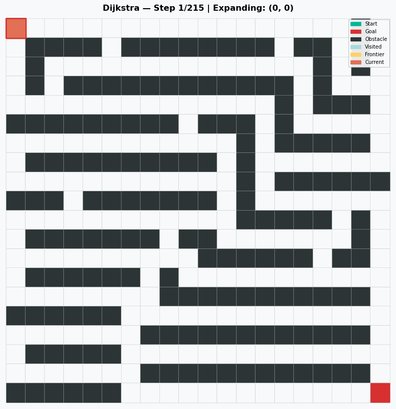
关键观察:Dijkstra 不考虑目标方向,会均匀探索所有可达区域,包括偏离目标的死胡同。在上图中,它扩展了 **215 个节点**才找到目标。
2.3 A* 搜索算法
A* 搜索是启发式搜索的经典算法,结合了 Dijkstra 算法和贪婪最佳优先搜索的优点。
算法原理
A* 算法:
f(n) = g(n) + h(n)

其中:
- g(n):从初始状态到 n 的实际代价
- h(n):从 n 到目标的估计代价(启发函数)
- f(n):总估计代价

性质:
- 如果 h(n) 是可采纳的(不高估),A* 是最优的
- 如果 h(n) 是一致的(满足三角不等式),A* 是高效的
- 当 h(n) = 0 时,A* 退化为 Dijkstra 算法
- 当 h(n) >> g(n) 时,A* 退化为贪婪最佳优先搜索
核心思想
A* 的关键创新是在 Dijkstra 的基础上加入了**启发函数 h(n)**,引导搜索朝目标方向前进。它不是盲目地均匀扩展,而是优先探索"看起来最有希望"的节点。
Dijkstra:  f(n) = g(n)           → 均匀扩展,不考虑方向
A*:        f(n) = g(n) + h(n)    → 有方向性,优先靠近目标的节点
Greedy:    f(n) = h(n)           → 只看方向,不保证最优
完整实现
import heapq

def a_star_search(problem, heuristic):
    """
    A* 搜索算法

    参数:
    problem: 规划问题
    heuristic: 启发函数 h(n) → 估计到目标的代价

    返回:
    plan: 动作序列(最优解),或 None(无解)
    """
    start = problem.initial_state
    goal = problem.goal_state

    # 优先队列:(f值, 状态)
    frontier = [(heuristic(start), start)]
    explored = set()
    g_score = {start: 0}
    parent = {start: None}
    action_taken = {start: None}

    while frontier:
        f, state = heapq.heappop(frontier)

        if state in explored:
            continue
        explored.add(state)

        if problem.is_goal(state):
            plan = []
            while state is not None:
                if action_taken[state] is not None:
                    plan.append(action_taken[state])
                state = parent[state]
            return plan[::-1]

        for action in problem.get_applicable_actions(state):
            new_state = action.apply(state)
            new_g = g_score[state] + action.cost

            if new_state not in g_score or new_g < g_score[new_state]:
                g_score[new_state] = new_g
                f = new_g + heuristic(new_state)
                heapq.heappush(frontier, (f, new_state))
                parent[new_state] = state
                action_taken[new_state] = action.name

    return None  # 无解


# 使用示例
def manhattan_heuristic(goal):
    """返回一个曼哈顿距离启发函数"""
    def h(state):
        return abs(state[0] - goal[0]) + abs(state[1] - goal[1])
    return h

problem = GridWorldProblem(grid, start=(0, 0), goal=(4, 7))
heuristic = manhattan_heuristic((4, 7))
plan = a_star_search(problem, heuristic)
print(f"A* 找到路径: {plan}")
print(f"路径长度: {len(plan)} 步")
A* 的搜索过程
同样的 20×20 网格,A* 通过启发函数引导搜索方向,大幅减少了探索的节点数。
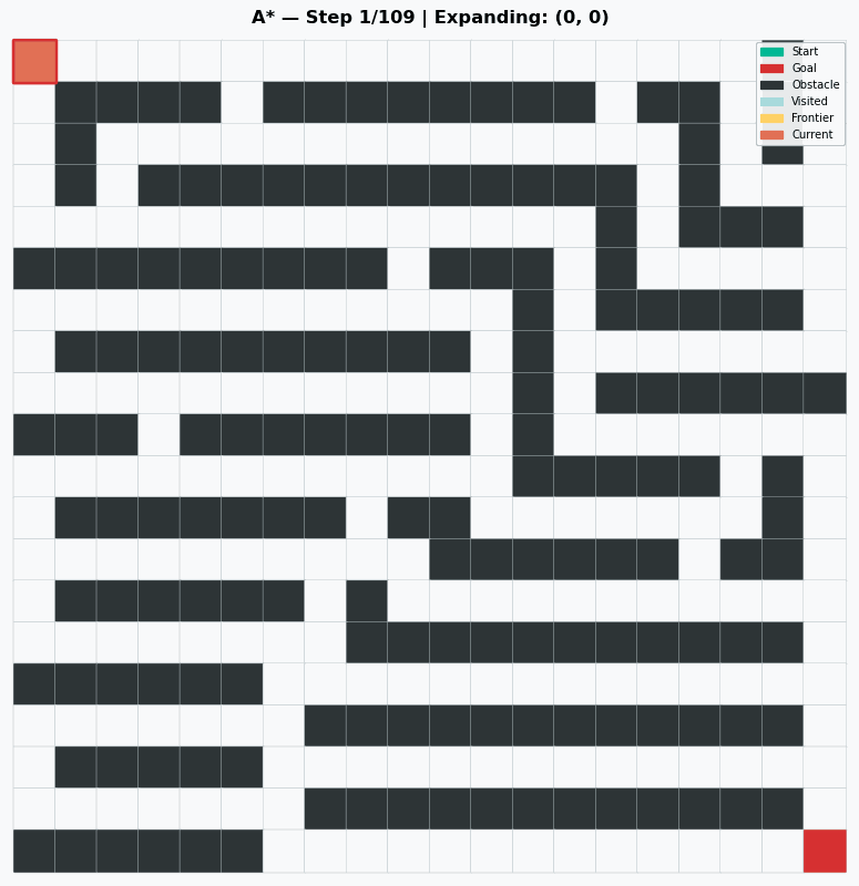
关键观察:A* 优先向目标方向扩展,避开了偏离目标的死胡同。在上图中,它只扩展了 109 个节点**就找到了目标——比 Dijkstra 的 215 个节点少了 **49%。
2.4 Dijkstra vs A* 对比
| 特性 | Dijkstra | A* |
|---|---|---|
| 启发函数 | 无(h(n) = 0) | 有(h(n) ≥ 0) |
| 搜索方向 | 均匀扩展,无方向性 | 有方向性,优先靠近目标 |
| 最优性 | ✅ 保证最优 | ✅ 当 h(n) 可采纳时 |
| 完整性 | ✅ 有解必找到 | ✅ 有解必找到 |
| 扩展节点数 | 多(探索所有可达区域) | 少(只探索有希望的区域) |
| 适用场景 | 无启发信息时 | 有好的启发函数时 |
| 时间复杂度 | O((V+E) log V) | 取决于 h(n) 的质量 |
直观理解
想象你在一个迷宫中找出口:
- Dijkstra:像一个水球从起点膨胀,均匀地向所有方向扩展,直到触达出口。
- 优点:不会错过任何捷径
-
缺点:浪费时间探索明显不对的方向
-
A*:像一个有方向感的人,知道出口大概在哪个方向,优先朝那个方向走,但不会忽略可能的捷径。
- 优点:效率高,少走弯路
- 缺点:需要一个好的"方向感"(启发函数)
启发函数的质量对 A* 的影响
# 不同启发函数对 A* 的影响

# 1. h(n) = 0  →  退化为 Dijkstra(最慢,但保证最优)
def h_zero(state, goal):
    return 0

# 2. 曼哈顿距离  →  4方向网格的可采纳启发(推荐)
def h_manhattan(state, goal):
    return abs(state[0] - goal[0]) + abs(state[1] - goal[1])

# 3. 欧几里得距离  →  任意方向移动的可采纳启发
def h_euclidean(state, goal):
    return ((state[0] - goal[0])**2 + (state[1] - goal[1])**2) ** 0.5

# 4. 切比雪夫距离  →  8方向网格的可采纳启发
def h_chebyshev(state, goal):
    return max(abs(state[0] - goal[0]), abs(state[1] - goal[1]))

# 5. 不可采纳的启发(高估)  →  可能不最优,但更快
def h_inadmissible(state, goal):
    return 2 * (abs(state[0] - goal[0]) + abs(state[1] - goal[1]))
启发函数的选择原则:
| 场景 | 推荐启发函数 | 原因 |
|---|---|---|
| 4方向网格(上下左右) | 曼哈顿距离 | 精确匹配移动方式 |
| 8方向网格(含对角线) | 切比雪夫距离 / 八方向距离 | 考虑对角线移动 |
| 连续空间 | 欧几里得距离 | 两点间直线最短 |
| 无信息 | h(n) = 0 | 退化为 Dijkstra |
2.5 启发函数的计算
def compute_heuristic_value(state, goal, obstacles, type='manhattan'):
    """
    计算启发函数值

    参数:
    state: 当前状态
    goal: 目标状态
    obstacles: 障碍物列表
    type: 启发函数类型

    返回:
    h: 启发值
    """
    if type == 'manhattan':
        # 曼哈顿距离
        h = abs(state[0] - goal[0]) + abs(state[1] - goal[1])

    elif type == 'euclidean':
        # 欧几里得距离
        h = np.sqrt((state[0] - goal[0])**2 + (state[1] - goal[1])**2)

    elif type == 'chebyshev':
        # 切比雪夫距离
        h = max(abs(state[0] - goal[0]), abs(state[1] - goal[1]))

    elif type == 'octile':
        # 八方向距离
        dx = abs(state[0] - goal[0])
        dy = abs(state[1] - goal[1])
        h = max(dx, dy) + (np.sqrt(2) - 1) * min(dx, dy)

    else:
        h = 0

    return h
3. 规划空间搜索
3.1 部分有序规划(POP)
部分有序规划不强制动作的完全顺序,允许动作之间的部分顺序。
class PartialOrderPlan:
    """部分有序规划"""

    def __init__(self):
        self.actions = []  # 动作列表
        self.ordering_constraints = []  # 顺序约束
        self.causal_links = []  # 因果链接
        self.open_preconditions = []  # 开放前置条件

    def add_action(self, action):
        """添加动作"""
        self.actions.append(action)

    def add_ordering_constraint(self, before, after):
        """添加顺序约束"""
        self.ordering_constraints.append((before, after))

    def add_causal_link(self, action, condition, supporter):
        """添加因果链接"""
        self.causal_links.append((action, condition, supporter))

    def is_consistent(self):
        """检查规划是否一致"""
        # 检查顺序约束是否有环
        # 检查因果链接是否被威胁
        return True

    def linearize(self):
        """线性化部分有序规划"""
        # 拓扑排序
        return self.topological_sort()

    def topological_sort(self):
        """拓扑排序"""
        # 构建邻接表
        graph = {a: [] for a in self.actions}
        in_degree = {a: 0 for a in self.actions}

        for before, after in self.ordering_constraints:
            graph[before].append(after)
            in_degree[after] += 1

        # 拓扑排序
        queue = [a for a in self.actions if in_degree[a] == 0]
        result = []

        while queue:
            action = queue.pop(0)
            result.append(action)

            for neighbor in graph[action]:
                in_degree[neighbor] -= 1
                if in_degree[neighbor] == 0:
                    queue.append(neighbor)

        return result

# 示例
plan = PartialOrderPlan()
plan.add_action('move_to_table')
plan.add_action('pick_up_block')
plan.add_action('move_to_target')
plan.add_action('put_down_block')

plan.add_ordering_constraint('move_to_table', 'pick_up_block')
plan.add_ordering_constraint('pick_up_block', 'move_to_target')
plan.add_ordering_constraint('move_to_target', 'put_down_block')

linear_plan = plan.linearize()
print("线性化规划:", linear_plan)
3.2 规划修复
规划修复是在现有规划的基础上进行修改,以解决规划失败的问题。
def repair_plan(plan, problem, max_repairs=10):
    """
    修复规划

    参数:
    plan: 现有规划
    problem: 规划问题
    max_repairs: 最大修复次数

    返回:
    repaired_plan: 修复后的规划
    """
    current_plan = plan.copy()

    for _ in range(max_repairs):
        # 验证规划
        if validate_plan(current_plan, problem):
            return current_plan

        # 识别失败点
        failure_point = find_failure_point(current_plan, problem)

        if failure_point is None:
            return None  # 无法修复

        # 选择修复策略
        repair_action = choose_repair_action(failure_point, problem)

        if repair_action is None:
            return None  # 无法修复

        # 插入修复动作
        current_plan = insert_repair_action(current_plan, repair_action, failure_point)

    return None  # 超过最大修复次数

def validate_plan(plan, problem):
    """验证规划"""
    state = problem.initial_state

    for action_name in plan:
        # 找到对应的动作
        action = find_action(action_name, problem)

        if action is None:
            return False

        # 检查动作是否可应用
        if not action.is_applicable(state):
            return False

        # 应用动作
        state = action.apply(state)

    # 检查是否达到目标
    return problem.is_goal(state)

def find_failure_point(plan, problem):
    """查找失败点"""
    state = problem.initial_state

    for i, action_name in enumerate(plan):
        action = find_action(action_name, problem)

        if action is None or not action.is_applicable(state):
            return i

        state = action.apply(state)

    return None
4. PDDL(规划领域定义语言)
4.1 PDDL 基础
PDDL 是用于描述规划问题的标准语言。
;; 定义领域
(define (domain grid-world)
  (:requirements :strips :typing)

  (:types
    location
  )

  (:predicates
    (robot-at ?loc - location)
    (adjacent ?from ?to - location)
    (blocked ?loc - location)
  )

  (:action move
    :parameters (?from ?to - location)
    :precondition (and
      (robot-at ?from)
      (adjacent ?from ?to)
      (not (blocked ?to))
    )
    :effect (and
      (not (robot-at ?from))
      (robot-at ?to)
    )
  )
)
4.2 PDDL 问题描述
;; 定义问题
(define (problem grid-world-problem)
  (:domain grid-world)

  (:objects
    loc-0-0 loc-0-1 loc-0-2
    loc-1-0 loc-1-1 loc-1-2
    loc-2-0 loc-2-1 loc-2-2 - location
  )

  (:init
    (robot-at loc-0-0)
    (adjacent loc-0-0 loc-0-1)
    (adjacent loc-0-1 loc-0-2)
    (adjacent loc-0-0 loc-1-0)
    (adjacent loc-1-0 loc-2-0)
    ;; ... 更多相邻关系
    (blocked loc-1-1)
  )

  (:goal
    (robot-at loc-2-2)
  )
)
4.3 PDDL 解析器
class PDDLParser:
    """PDDL 解析器"""

    def __init__(self):
        self.domain = None
        self.problem = None

    def parse_domain(self, domain_str):
        """解析领域定义"""
        # 简化解析
        lines = domain_str.strip().split('\n')

        domain = {
            'name': '',
            'requirements': [],
            'types': {},
            'predicates': [],
            'actions': []
        }

        current_section = None
        current_action = None

        for line in lines:
            line = line.strip()

            if line.startswith('(define (domain'):
                domain['name'] = line.split('(')[2].split(')')[0]

            elif ':requirements' in line:
                domain['requirements'] = line.split(':')[1].strip().split()

            elif ':types' in line:
                current_section = 'types'

            elif ':predicates' in line:
                current_section = 'predicates'

            elif ':action' in line:
                current_section = 'action'
                action_name = line.split(':')[1].strip()
                current_action = {'name': action_name}

            elif current_section == 'action':
                if ':parameters' in line:
                    current_action['parameters'] = line.split(':')[1].strip()
                elif ':precondition' in line:
                    current_action['precondition'] = line.split(':')[1].strip()
                elif ':effect' in line:
                    current_action['effect'] = line.split(':')[1].strip()
                    domain['actions'].append(current_action)
                    current_action = None

        self.domain = domain
        return domain

    def parse_problem(self, problem_str):
        """解析问题定义"""
        # 类似解析领域定义
        pass
5. 实践练习
练习 1:实现前向搜索
# 实现前向搜索算法
def forward_search_exercise():
    # 创建网格世界
    grid = [
        [0, 0, 0, 0, 0],
        [0, 1, 1, 0, 0],
        [0, 0, 0, 0, 0],
        [0, 0, 1, 1, 0],
        [0, 0, 0, 0, 0]
    ]

    # 创建问题
    problem = GridWorldProblem(grid, (0, 0), (4, 4))

    # 使用 A* 搜索
    heuristic = HeuristicFunction((4, 4), type='manhattan')
    plan = a_star_search(problem, heuristic)

    print("规划结果:", plan)
    return plan
练习 2:实现部分有序规划
# 实现部分有序规划
def pop_exercise():
    # 创建规划
    plan = PartialOrderPlan()

    # 添加动作
    plan.add_action('goto_door')
    plan.add_action('open_door')
    plan.add_action('goto_room')
    plan.add_action('pickup_object')

    # 添加顺序约束
    plan.add_ordering_constraint('goto_door', 'open_door')
    plan.add_ordering_constraint('open_door', 'goto_room')
    plan.add_ordering_constraint('goto_room', 'pickup_object')

    # 线性化
    linear_plan = plan.linearize()
    print("线性化规划:", linear_plan)

    return linear_plan
练习 3:实现 PDDL 解析器
# 实现 PDDL 解析器
def pddl_exercise():
    domain_str = """
    (define (domain grid-world)
      (:requirements :strips)

      (:predicates
        (robot-at ?x ?y)
        (blocked ?x ?y)
      )

      (:action move-up
        :parameters (?x ?y)
        :precondition (and (robot-at ?x ?y) (not (blocked ?x (+ ?y 1))))
        :effect (and (not (robot-at ?x ?y)) (robot-at ?x (+ ?y 1)))
      )
    )
    """

    parser = PDDLParser()
    domain = parser.parse_domain(domain_str)

    print("解析的领域:", domain)
    return domain
6. 常见问题
1. 搜索空间爆炸
问题:状态空间太大,搜索效率低
解决方案: - 使用启发式函数 - 使用分层规划 - 使用剪枝技术
2. 启发函数设计
问题:如何设计好的启发函数?
解决方案: - 使用放松问题(relaxed problem) - 使用模式数据库(pattern database) - 使用学习的方法
3. 规划失败
问题:找不到可行规划
解决方案: - 检查问题定义 - 增加搜索深度 - 使用规划修复
下一步
参考资源
- Acting, Planning, and Learning - Chapter 3
- Planning Algorithms
- PDDL - Planning Domain Definition Language